data(credit_data, package = "modeldata")
credit <- as_tibble(credit_data)“Which model should we use?” comes up in almost every project, and it is usually answered badly. Someone picks a random forest because it worked last time. Someone else wants gradient boosting because it wins Kaggle. A third person asks for logistic regression because the risk committee can read it.
Each of them has a point. None of them has evidence, because the models were never compared on the same data, with the same resamples, under the same metric.
A model leaderboard fixes that: one table where every candidate was trained and evaluated under identical rules, ranked by a metric chosen before looking. The tidymodels package for this is workflowsets. This post builds a leaderboard for a credit approval problem and then goes one step further: it turns the winner into a decision that makes money.
What you need
- Basic tidymodels: recipes, model specs and workflows. If you have run
fit_resamples()once, you are fine. - No private data. The example uses
credit_data, which ships with the modeldata package. - One coffee. The full race takes about six minutes on three cores. Everything is seeded.
The tooling changed in 2025 and 2026. tune 2.x dropped foreach in favour of mirai and future, added tunable postprocessors through the tailor package, and renamed the .config identifiers. Older tutorials still run, but their output looks different.
The five steps
- Split once, resample once. Every model sees the same folds.
- Define the candidates. A few preprocessors and a few models.
- Cross them into a workflow set. Each combination becomes one row of a tibble.
- Race them. Tune every workflow with the same budget and drop bad candidates early.
- Read the leaderboard, then decide. Rank, check whether the winner is really better, and pick the cutoff the business needs.
Steps 1 to 4 are mechanics. Step 5 is where the value is, and where most leaderboards stop too early.
The problem: who gets the loan?
| Variable | Meaning |
|---|---|
| Status | Outcome: good (repaid) or bad (defaulted) |
| Seniority | Years in the current job |
| Home | Housing situation (owner, rent, parents, …) |
| Time | Loan term in months |
| Age | Age of the applicant |
| Marital | Marital status |
| Records | Whether the applicant has prior bad records |
| Job | Type of employment (fixed, freelance, part-time, …) |
| Expenses | Monthly expenses |
| Income | Monthly income |
| Assets | Total assets |
| Debt | Outstanding debt |
| Amount | Loan amount requested |
| Price | Price of the good being financed |
The data are 4,454 consumer credit applications from a Spanish lender. The predictors are what an underwriter asks for. The bad rate is 28.2%: high for a credit book, which makes the decision interesting. Approve everyone and you lose money; decline everyone and you have no business.
The question for the model is not “is this applicant bad?” but “should we approve this loan?”. That distinction comes back in step 5.
Step 1: split once, resample once
set.seed(2026)
credit_split <- initial_split(credit, prop = 0.8, strata = Status)
credit_train <- training(credit_split)
credit_test  <- testing(credit_split)

set.seed(2026)
credit_folds <- vfold_cv(credit_train, v = 10, strata = Status)
The test set stays locked until the end. All comparisons happen on the ten folds, and every model gets the same ten. Models tuned on different resamples are not comparable: differences between folds leak into differences between models.
Step 2: two preprocessors, five models
The first preprocessor does the minimum: impute, encode categories, drop constant columns, normalise.
rec_plain <- recipe(Status ~ ., data = credit_train) |>
  step_impute_median(all_numeric_predictors()) |>
  step_unknown(all_nominal_predictors()) |>
  step_dummy(all_nominal_predictors()) |>
  step_zv(all_predictors()) |>
  step_normalize(all_numeric_predictors())
The second adds what a credit analyst computes by hand. Underwriting runs on ratios: how much of the price is financed, how many months of income the loan represents, how much income is already committed to debt, and how much the instalment will take.
rec_ratios <- recipe(Status ~ ., data = credit_train) |>
  step_impute_median(all_numeric_predictors()) |>
  step_unknown(all_nominal_predictors()) |>
  step_mutate(
    loan_to_value     = Amount / pmax(Price, 1),
    amount_to_income  = Amount / pmax(Income, 1),
    debt_to_income    = Debt / pmax(Income, 1),
    payment_to_income = (Amount / pmax(Time, 1)) / pmax(Income, 1)
  ) |>
  step_log(Income, Assets, Debt, Amount, Price, offset = 1) |>
  step_dummy(all_nominal_predictors()) |>
  step_zv(all_predictors()) |>
  step_normalize(all_numeric_predictors())
Having both in the leaderboard answers a second question for free: does domain feature engineering still matter when tree ensembles can, in theory, learn the ratios themselves?
The five models are the usual suspects for tabular data. Each tunes its main parameters. The number of trees is fixed to keep the race short.
glmnet_spec <- logistic_reg(penalty = tune(), mixture = tune()) |>
  set_engine("glmnet")

rf_spec <- rand_forest(mtry = tune(), min_n = tune(), trees = 500) |>
  set_engine("ranger") |>
  set_mode("classification")

xgb_spec <- boost_tree(trees = 500, learn_rate = tune(),
                       tree_depth = tune(), min_n = tune()) |>
  set_engine("xgboost") |>
  set_mode("classification")

lgb_spec <- boost_tree(trees = 500, learn_rate = tune(),
                       tree_depth = tune(), min_n = tune()) |>
  set_engine("lightgbm") |>
  set_mode("classification")

nnet_spec <- mlp(hidden_units = tune(), penalty = tune(), epochs = 200) |>
  set_engine("nnet") |>
  set_mode("classification")
LightGBM is not a native parsnip engine. The bonsai package adds it; loading bonsai is all it takes.
Step 3: cross them into a workflow set
credit_set <- workflow_set(
  preproc = list(plain = rec_plain, ratios = rec_ratios),
  models  = list(logistic = glmnet_spec, rf = rf_spec, xgboost = xgb_spec,
                 lightgbm = lgb_spec, nnet = nnet_spec),
  cross = TRUE
)| Workflow id | Preprocessor | Model type | Engine |
|---|---|---|---|
| plain_logistic | plain | logistic_reg | glmnet |
| plain_rf | plain | rand_forest | ranger |
| plain_xgboost | plain | boost_tree | xgboost |
| plain_lightgbm | plain | boost_tree | lightgbm |
| plain_nnet | plain | mlp | nnet |
| ratios_logistic | ratios | logistic_reg | glmnet |
| ratios_rf | ratios | rand_forest | ranger |
| ratios_xgboost | ratios | boost_tree | xgboost |
| ratios_lightgbm | ratios | boost_tree | lightgbm |
| ratios_nnet | ratios | mlp | nnet |
Two preprocessors times five models gives ten workflows, each named preprocessor_model. Per-workflow settings live in the option column. One default needs fixing: the dials range for learn_rate goes down to \(10^{-10}\), which with 500 trees means a model that barely moves. Both boosting engines get a tighter range.
boost_params <- xgb_spec |>
  extract_parameter_set_dials() |>
  update(learn_rate = learn_rate(c(-2.5, -0.5)))

for (id in c("plain_xgboost", "ratios_xgboost", "plain_lightgbm", "ratios_lightgbm")) {
  credit_set <- option_add(credit_set, param_info = boost_params, id = id)
}
Step 4: race them
A full grid search fits every candidate on every fold: 20 candidates times 10 folds times 10 workflows is 2,000 fits before anything is ranked. Racing avoids most of that. After a few folds it runs an ANOVA on the per-fold metrics and drops every candidate already significantly worse than the leader. Only survivors see the remaining folds.
The metric set matters: racing eliminates on the first metric, so it goes first.
credit_metrics <- metric_set(roc_auc, brier_class, sensitivity, specificity)Parallel processing in tune 2.x is one line with mirai. Three workers is conservative for a 16 GB laptop; raise it if you have the memory.
mirai::daemons(3)

set.seed(2026)
credit_res <- credit_set |>
  workflow_map(
    "tune_race_anova",
    resamples = credit_folds,
    grid = 20,
    metrics = credit_metrics,
    control = control_race(save_pred = TRUE, save_workflow = TRUE),
    seed = 2026
  )

mirai::daemons(0)
The result column now holds one racing result per workflow. This is what the race looked like for the boosted trees with ratio features:
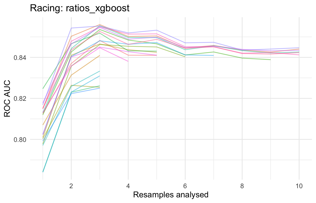
Each line is a candidate. Most are eliminated after the third fold; a handful run all ten. The time saved goes into more workflows, which is the right trade.
Step 5a: the leaderboard
rank_results() is the leaderboard. With select_best = TRUE it keeps the best configuration of each workflow, so there is one row per workflow.
survivors <- credit_res |>
  mutate(candidates = map_int(result, \(x) {
    collect_metrics(x) |> filter(.metric == "roc_auc") |> nrow()
  })) |>
  select(wflow_id, candidates)

leaderboard <- rank_results(credit_res, rank_metric = "roc_auc", select_best = TRUE) |>
  select(wflow_id, .metric, mean, std_err, rank) |>
  pivot_wider(names_from = .metric, values_from = c(mean, std_err)) |>
  left_join(survivors, by = "wflow_id") |>
  separate_wider_delim(wflow_id, "_", names = c("preprocessor", "model"),
                       cols_remove = FALSE) |>
  arrange(rank)

best_id  <- leaderboard$wflow_id[1]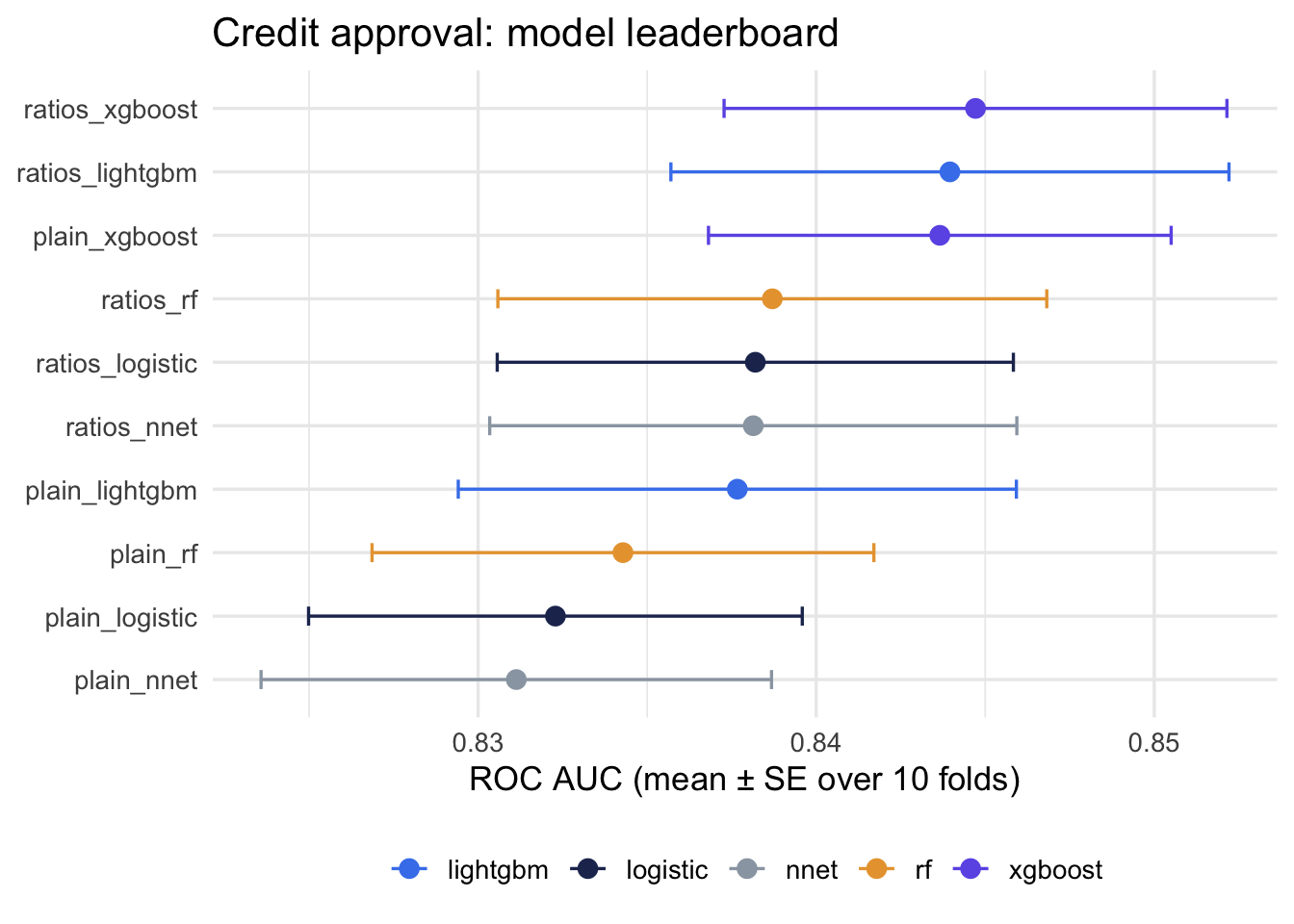
Three things stand out.
- The ratio features helped every model. Each
ratios_*row sits above itsplain_*twin, including the tree ensembles. On 3,500 rows, “can learn it in theory” is not the same as learning it. - The top three are a tie. The error bars of ratios_xgboost, ratios_lightgbm and plain_xgboost overlap almost entirely.
- Sensitivity is low everywhere. About half of the bad loans are missed at the default 50% cutoff. That is the wrong cutoff, not a bad model. Step 5c fixes it.
Step 5b: is the winner really better?
A leaderboard ranks means. But every model was evaluated on the same ten folds, which makes this paired data. The fair comparison is the fold-by-fold gap to the leader with its own standard error, exactly as a paired t-test would do it. Same logic as the decision flow for hypothesis tests.
best_configs <- rank_results(credit_res, rank_metric = "roc_auc", select_best = TRUE) |>
  filter(.metric == "roc_auc") |>
  select(wflow_id, .config)

fold_auc <- collect_metrics(credit_res, summarize = FALSE) |>
  filter(.metric == "roc_auc") |>
  inner_join(best_configs, by = c("wflow_id", ".config")) |>
  select(wflow_id, id, auc = .estimate)

paired <- fold_auc |>
  left_join(fold_auc |> filter(wflow_id == best_id) |> select(id, best_auc = auc),
            by = "id") |>
  mutate(gap = best_auc - auc) |>
  group_by(wflow_id) |>
  summarise(mean_gap = mean(gap), se = sd(gap) / sqrt(n()), .groups = "drop") |>
  filter(wflow_id != best_id) |>
  mutate(lower = mean_gap - 2 * se,
         upper = mean_gap + 2 * se,
         verdict = if_else(lower > 0, "Leader is better", "Statistical tie"))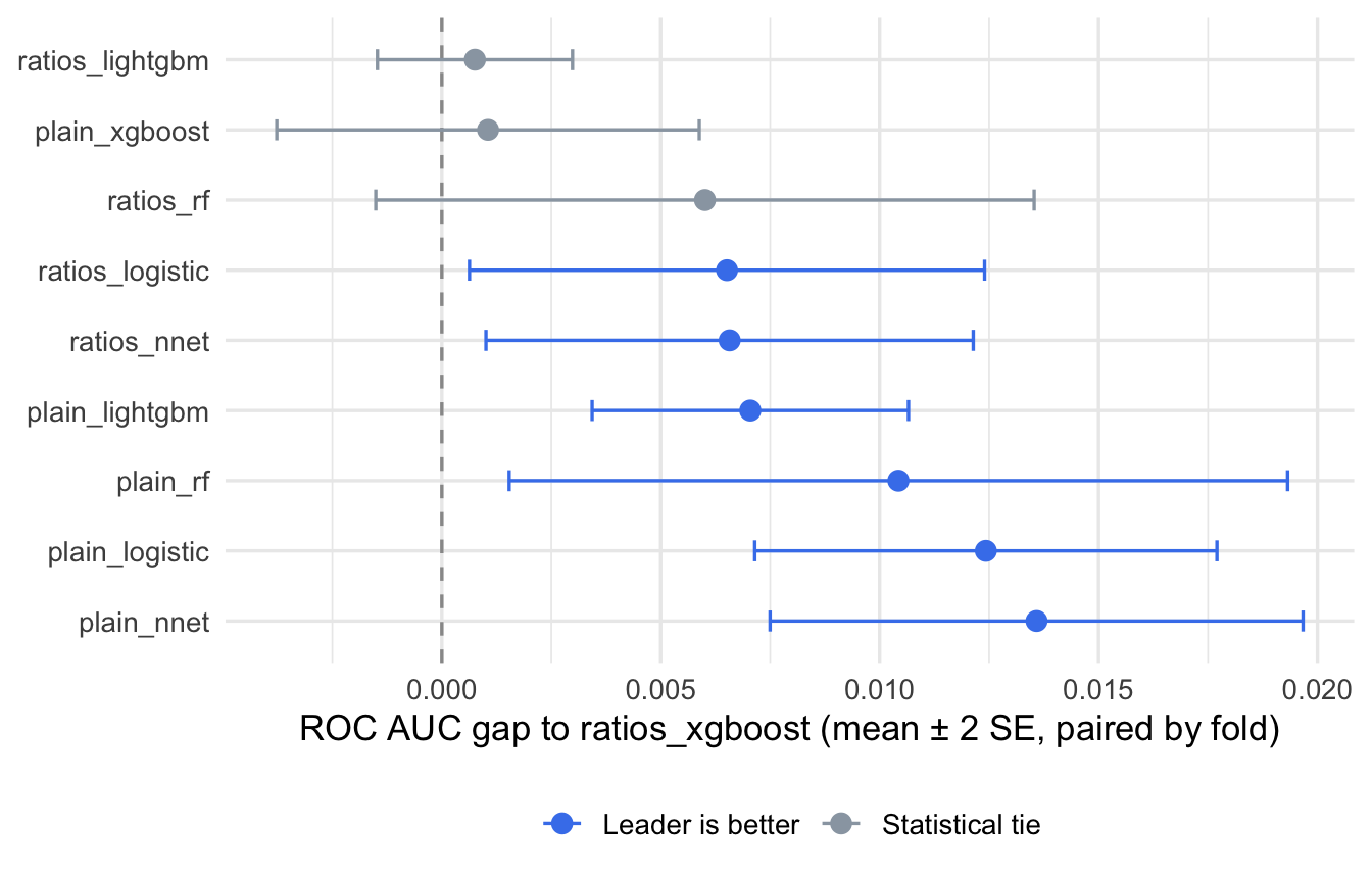
Only the models whose interval excludes zero are convincingly worse than the leader. 3 of the nine are ties: ratios_lightgbm, plain_xgboost, and ratios_rf. The honest reading is not “xgboost wins”. It is “with ratio features, both boosting engines and the random forest are indistinguishable at this sample size, and the logistic regression is just behind”.
When the top is a tie, the deciding factors stop being statistical. Which model can the risk committee read? Which has fewer moving parts in production? glmnet is a dozen coefficients and no external binary. LightGBM is a compiled library with its own versioning. Those questions decide the tie.
For this post the leader stays. Its winning configuration is worth a look:
best_params <- credit_res |>
  extract_workflow_set_result(best_id) |>
select_best(metric = "roc_auc")| min_n | tree_depth | learn_rate |
|---|---|---|
| 30 | 1 | 0.074 |
Trees of depth 1 with a small learning rate. A depth-1 ensemble is a sum of single splits: an additive model with automatic binning. It is closer to the logistic regression than its name suggests, which explains why the two sit so near each other.
Step 5c: from leaderboard to decision
The leaderboard ranks probability quality. The business needs a yes or no per application. The cutoff that converts one into the other should come from the economics, not from the default 0.5.
The economics here are simple and stated up front. A repaid loan earns about 10% of its amount in interest margin. A defaulted loan loses about 60% of its amount after recovery. A declined application earns and loses nothing.
margin_good <- 0.10
loss_bad    <- 0.60
break_even  <- margin_good / (margin_good + loss_bad)

credit_pnl <- function(data, approve) {
  data |>
    mutate(
      approve = approve,
      pnl = case_when(
        !approve         ~ 0,
        Status == "good" ~  margin_good * Amount,
        TRUE             ~ -loss_bad * Amount
      )
    ) |>
    summarise(
      approval_rate     = mean(approve),
      bad_rate_approved = mean(Status[approve] == "bad"),
      profit_per_1000   = 1000 * sum(pnl) / n()
    )
}
Under these numbers a loan is worth approving only if its probability of default is below 14.3%, the break-even point where \(0.10 \cdot (1 - p) = 0.60 \cdot p\). The portfolio’s base rate is twice that. A 50% cutoff is guaranteed to approve loans that lose money.
The out-of-fold predictions saved during the race are the right place to check this. They were made on data the model had not seen, and they are already computed.
oof <- credit_res |>
  extract_workflow_set_result(best_id) |>
  collect_predictions(parameters = best_params) |>
  left_join(credit_train |> mutate(.row = row_number()) |> select(.row, Amount),
            by = ".row")

profit_curve <- map(seq(0.05, 0.95, by = 0.05), \(th) {
  credit_pnl(oof, approve = oof$.pred_bad < th) |> mutate(threshold = th, .before = 1)
}) |>
  list_rbind()

best_threshold <- profit_curve |> slice_max(profit_per_1000, n = 1) |> pull(threshold)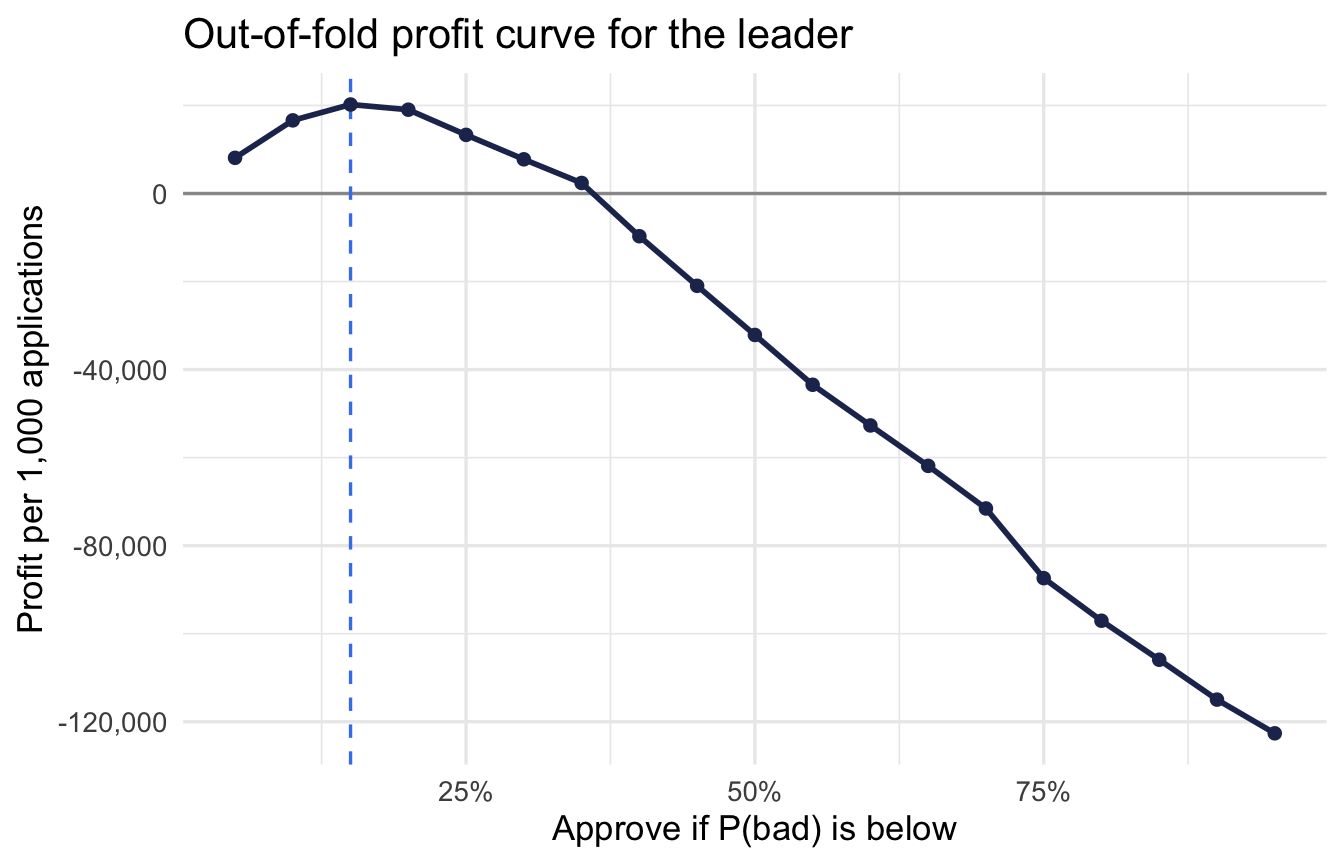
| Threshold | Approval rate | Bad rate among approved | Profit per 1,000 |
|---|---|---|---|
| 10.0% | 27.0% | 3.3% | 16,618 |
| 15.0% | 39.3% | 5.1% | 20,219 |
| 20.0% | 49.3% | 7.5% | 19,041 |
| 30.0% | 63.5% | 11.4% | 7,771 |
| 50.0% | 81.3% | 18.2% | -32,131 |
The curve peaks at 15%, close to the break-even point and far from 50%. At 50% the lender approves four out of five applications and loses money. At 15% it approves fewer than half and the book is profitable. Same model, same probabilities, a different sentence in the policy document.
Putting the threshold inside the model
This is where tailor earns its place. A postprocessor is part of the workflow, so the cutoff travels with the model. Whoever calls predict() in production gets the class decision the business agreed on, not the 50% default plus a note in the documentation.
final_wf <- credit_res |>
  extract_workflow(best_id) |>
  finalize_workflow(best_params) |>
  add_tailor(
    tailor() |>
      adjust_probability_threshold(threshold = best_threshold)
  )

final_fit <- last_fit(final_wf, credit_split, metrics = credit_metrics)| Metric | Estimate |
|---|---|
| sensitivity | 0.908 |
| specificity | 0.545 |
| roc_auc | 0.849 |
| brier_class | 0.138 |
last_fit() trains on the full training set and evaluates once on the test set locked away in step 1. The ROC AUC matches the resampling estimate, so the leaderboard did not overfit the folds. Sensitivity and specificity swapped places compared with the leaderboard: the cutoff now says “decline unless clearly good”.
test_pred <- collect_predictions(final_fit) |>
left_join(credit |> mutate(.row = row_number()) |> select(.row, Amount), by = ".row")| Actually bad | Actually good | |
|---|---|---|
| Predicted bad | 228 | 291 |
| Predicted good | 23 | 349 |
The .pred_class column already reflects the 15% cutoff, because the postprocessor ran inside last_fit(). Most bad loans are now caught, at the price of declining a good share of the good ones.
test_pnl <- bind_rows(
  `Approve everyone`                  = credit_pnl(test_pred, rep(TRUE, nrow(test_pred))),
  `Model, default 50% cutoff`         = credit_pnl(test_pred, test_pred$.pred_bad < 0.5),
  `Model, tuned cutoff (in workflow)` = credit_pnl(test_pred, test_pred$.pred_class == "good"),
  .id = "policy"
)| Policy | Approval rate | Bad rate among approved | Profit per 1,000 |
|---|---|---|---|
| Approve everyone | 100.0% | 28.2% | -120,431 |
| Model, default 50% cutoff | 82.4% | 18.5% | -20,909 |
| Model, tuned cutoff (in workflow) | 41.8% | 6.2% | 21,301 |
The sentence for the credit committee is the last row. Approve the 42% of applications the model is confident about, keep the bad rate on the approved book near 6%, and turn a loss-making portfolio into a profitable one. The AUC never appears in that sentence.
Reading leaderboards without fooling yourself
- Same folds or no comparison. The leaderboard is fair only because every workflow saw identical resamples. Never compare numbers from different
vfold_cv()calls. - Rank on the folds, confirm on the test set, once. Using the test set to choose between models turns it into one more fold and you lose your only honest estimate.
- Error bars first, rank second. A gap smaller than two standard errors is a tie. Let interpretability and operations decide ties.
- Pick the metric before the race. Racing eliminates on the first metric in the set. Change the order and you change who survives.
- Racing is a heuristic. A candidate that only shines with an unusual configuration can be dropped on the early folds. If a model surprises you by doing badly, rerun it alone with
tune_grid(). - Probability quality and decision quality are different problems. AUC and Brier measure the first; the cutoff and the cost matrix decide the second. A leaderboard that stops at AUC has done half the job.
- Record versions. tune 2.x changed the random streams, so results will not match objects made with tune 1.x.
Limitations
- The cost assumptions (10% margin, 60% loss) are illustrative. In a real desk they come from finance and differ by product. The method does not change; the numbers do.
- The threshold was chosen by looking at out-of-fold predictions. A stricter version tunes it inside the resampling with
adjust_probability_threshold(threshold = tune())and a custom profit metric. - Ten workflows is a small leaderboard. More preprocessors (interactions, splines, target encoding of
Job) or engines are just more rows, and racing keeps the cost reasonable. - Class imbalance was handled only through the cutoff. Resampling steps from the themis package could be a third preprocessor.
- The post ranks on a single metric. With several objectives, the desirability2 package ranks on a combination.
Cheat sheet
| Task | Function |
|---|---|
| Build the grid of preprocessors times models | workflow_set(preproc, models, cross = TRUE) |
| Change settings for one workflow | option_add(id = ..., param_info = ..., control = ...) |
| Tune or resample every workflow | workflow_map(fn, ...) with fn one of "tune_grid", "tune_race_anova", "fit_resamples" |
| Rank the results | rank_results(rank_metric = ..., select_best = TRUE) |
| Default leaderboard chart | autoplot(wf_set, metric = ..., select_best = TRUE) |
| Per-fold metrics for paired comparison | collect_metrics(wf_set, summarize = FALSE) |
| See how the race eliminated candidates | plot_race(extract_workflow_set_result(wf_set, id)) |
| Pull one workflow’s tuning result | extract_workflow_set_result(wf_set, id) |
| Pull the untrained workflow | extract_workflow(wf_set, id) |
| Best parameters and finalisation | select_best(), finalize_workflow() |
| Add a business cutoff to the workflow | add_tailor(tailor() \|> adjust_probability_threshold(...)) |
| Final fit and test-set evaluation | last_fit(split), collect_metrics(), collect_predictions() |
| Parallel resampling in tune 2.x | mirai::daemons(n) or future::plan("multisession") |
References and next steps
- Kuhn, M. & Silge, J. Tidy Modeling with R, chapter 15: Screening many models.
- The workflowsets vignette Tuning and comparing models and the reference for
rank_results(). - Kuhn, M., Couch, S., Hvitfeldt, E. & Frick, H. (2025). tune version 2.0.0: parallel processing with mirai and postprocessing with tailor. The April 2026 tidymodels releases cover tune 2.1.0 and yardstick 1.4.0.
- Kuhn, M. (2014). Futility analysis in the cross-validation of machine learning models. The paper behind
tune_race_anova(). - The
credit_datadocumentation in modeldata.
The natural follow-up is to stop choosing at all: the stacks package blends the top of a leaderboard into one ensemble, using the same workflow set as input. That is the next post in this series.